Exploring Dice Pools - A Probability Analysis

I’m currently designing my own tabletop RPG and considering using dice pools as the core mechanic. I believe that to effectively implement a dice mechanic, you first need to thoroughly understand it. So, I’ve analyzed various probability distributions related to dice pools, and plotted a few of them.

Definitions

For the purpose of this post, a dice pool is a mechanic where you roll a number of dice and count how many of them succeed based on a threshold value.

A dice pool system has the following properties:

Die Size - The type of die you are using (d6, d8, etc.)
Threshold - The minimum number rolled on a die that counts as a success. For example, a threshold of 4 means that rolling a 4 or higher counts as a success
Required Successes - The number of successes you need to roll for the test to be considered passed - how many dice need to roll over the treshold
Pool Size - The number of dice in your pool

Here, I’ve chosen to only consider six-sided dice, due to their popularity. Also, I find a pool of d6s more esthetically pleasing than a pool of other dice - d8s, for example.

Probability of Passing the Test

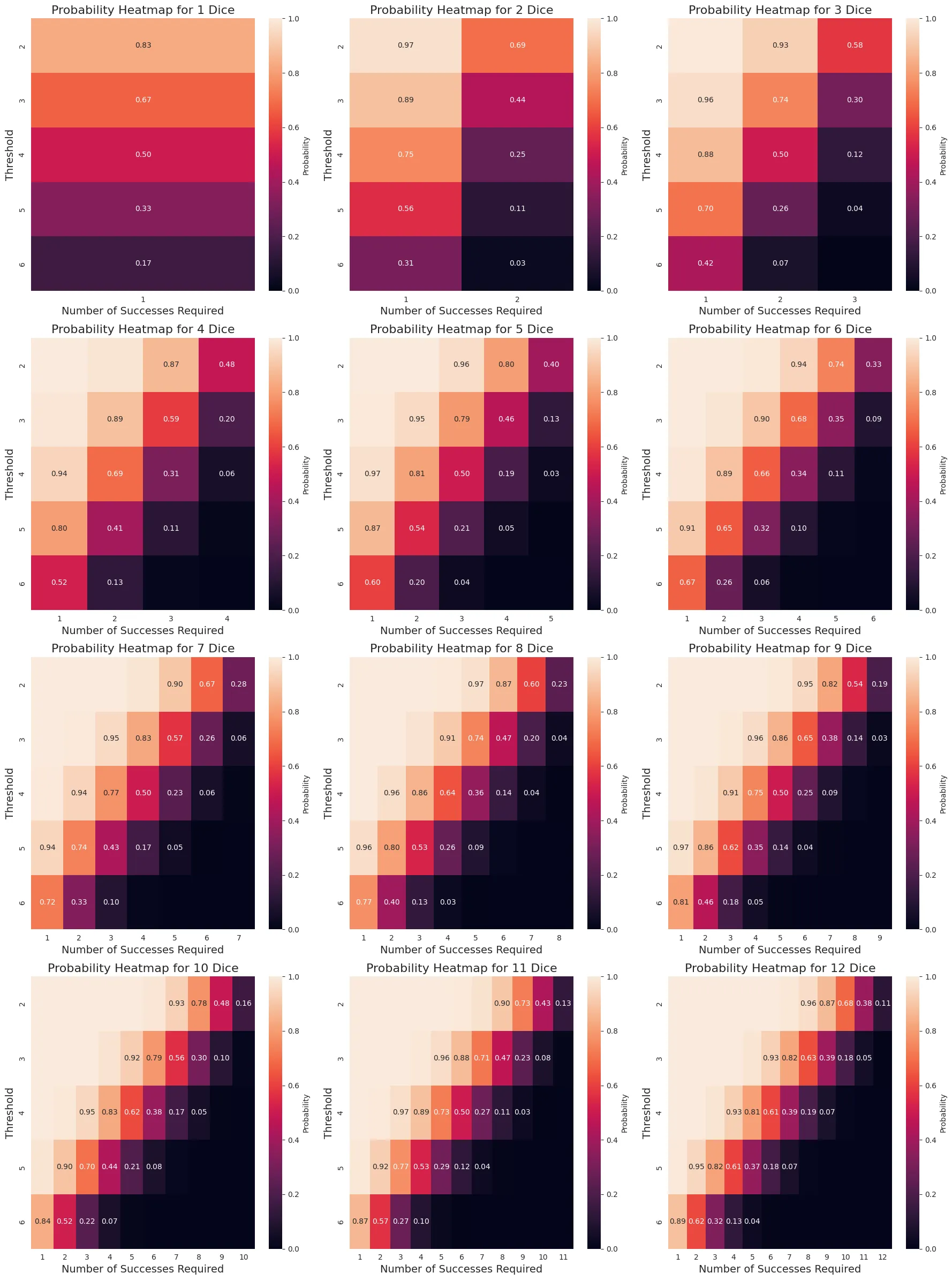
I’ve plotted the probabilities of passing a test for pool sizes ranging from 1 to 12 dice, with thresholds from 2 to 6, and required successes ranging from one up to the pool size (where every die would need to succeed).

Several interesting patterns emerge:

Many test configurations result in either near-certain success (probability close to 1) or near-certain failure (probability close to 0)
This becomes more pronounced with larger dice pools, where the majority of cases are either automatic failures or automatic successes
I’ll refer to these auto-fail/auto-pass cases as “trivial” tests
For a fixed threshold, there are surprisingly few significant, non-trivial test cases - typically around 6
With smaller pools, adjusting the difficulty diagonally (-1 threshold +1 required success, or +1 threshold -1 required success) results in nearly identical success probabilities

Analysing Difficulty Granularity

Dice pools are often criticized for offering less granular difficulty scaling than other dice systems.

Below, I’ve plotted the probabilities of passing different test configurations for each pool size, ordered from hardest to easiest. The label X:Y represents a test with Threshold X and Y required successes. When probabilities were too close together, I’ve only labeled the first test in the cluster.

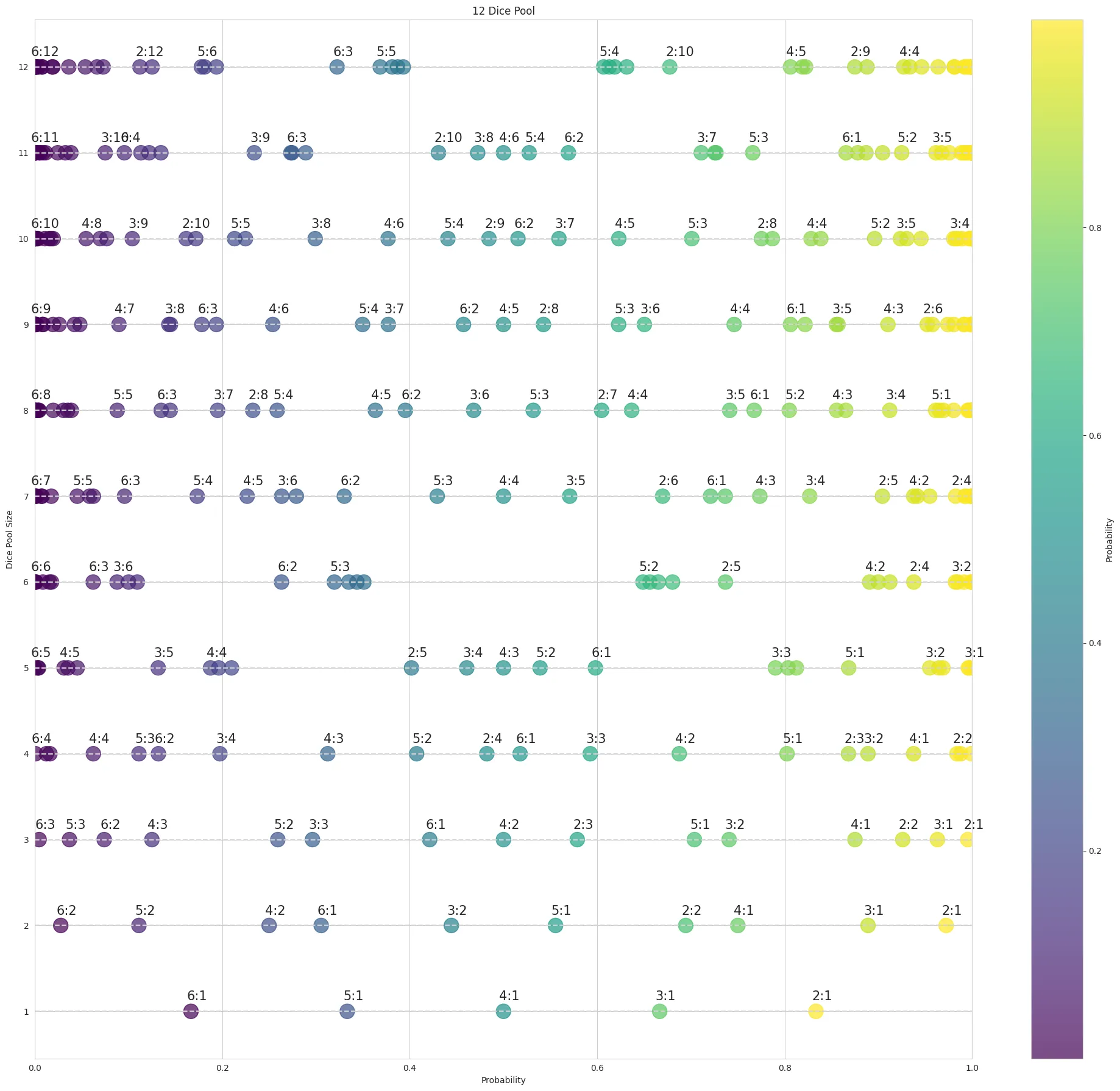
Key observations:

Most pool sizes show difficulty clusters that are roughly evenly distributed across the probability spectrum
However, their ordering is not intuitive - when rolling 7 dice, is 4:5 easier than 6:2?
Interesting patterns emerge with 6 and 12 dice, where test cases cluster more tightly together

My conclusion is that yes, you can make dice pools very granular, it would be, however, quite tricky.

Analysing Success Requirements and Thresholds

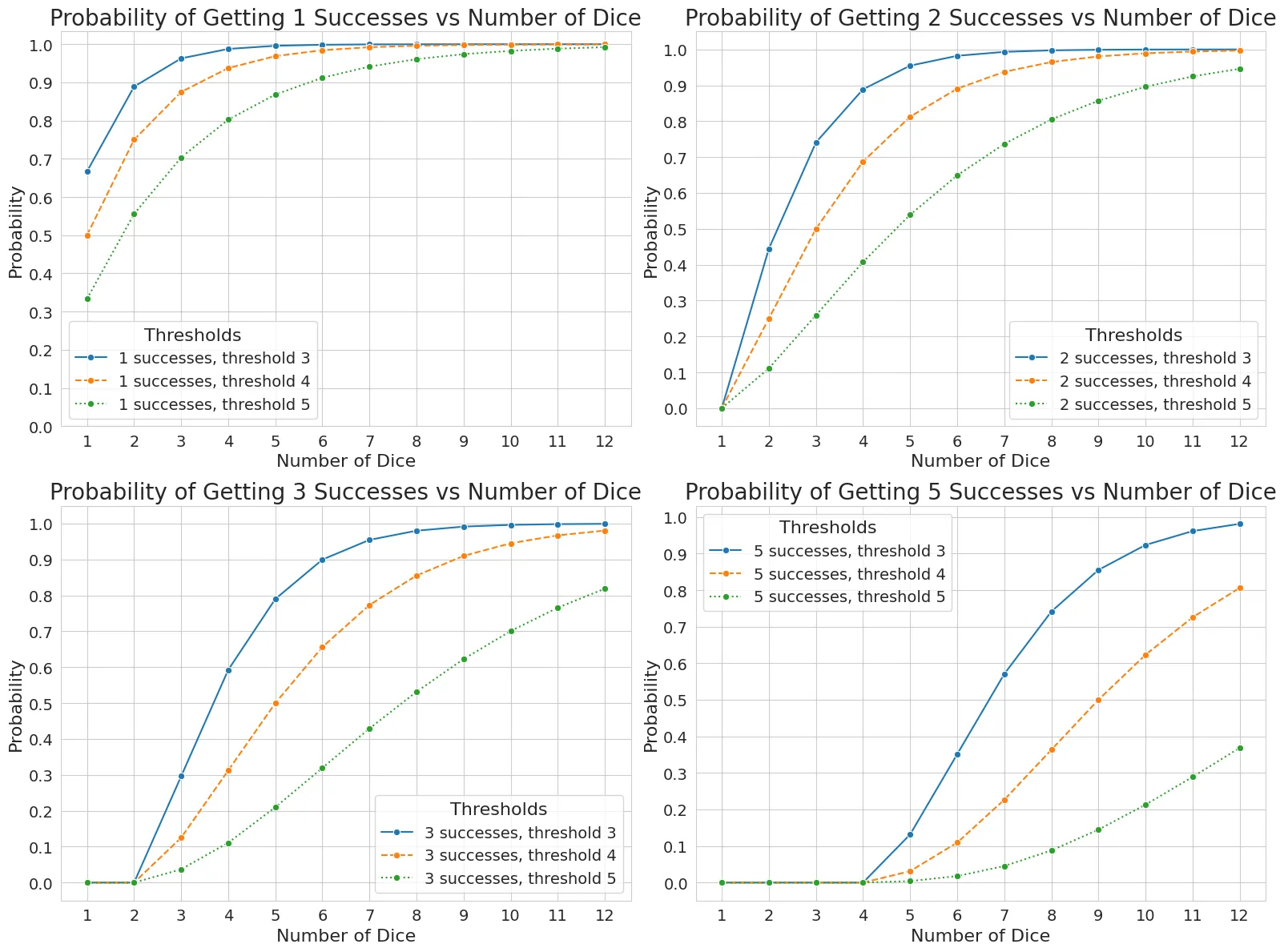
The above probabilities were calculated using a fixed threshold of 4.

Some key insights:

Changing the number of required successes produces non-linear changes in test difficulty
The impact is most significant when the required successes are close to the expected number of successes for a given pool size
For a threshold of 4, this occurs around half the pool size - adjusting the required successes has the greatest impact when that number is close to half the dice pool size
While the resulting probability changes may seem unpredictable, the variations are generally modest enough (0.12-0.17) that they won’t significantly impact casual gameplay

Opposed Tests

An opposed test occurs when two characters roll their respective dice pools and count successes, potentially with different thresholds. The test’s outcome is determined by the difference between the number of successes rolled by each party.

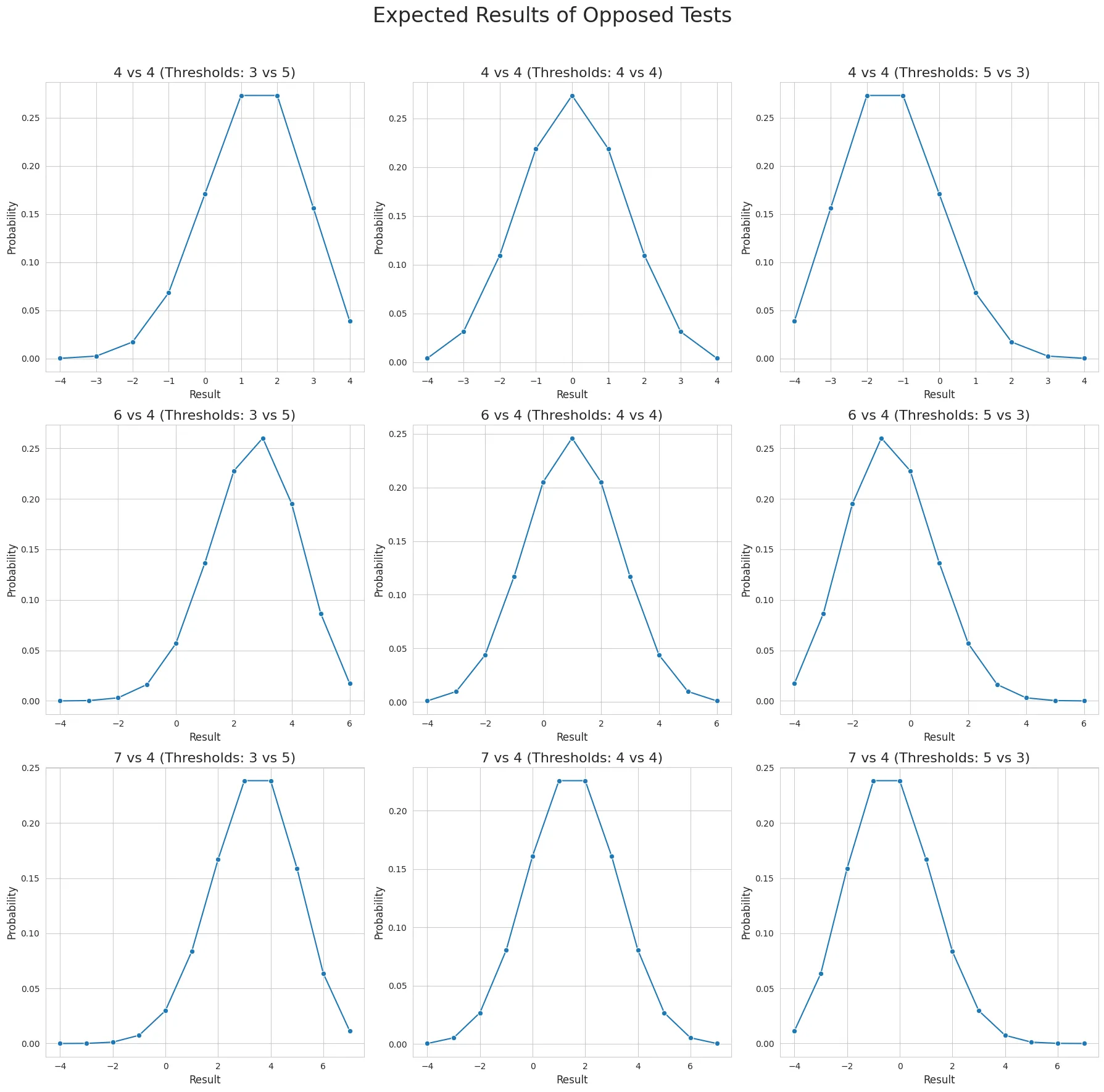
Dice pools demonstrate particularly predictable and intuitive behavior in opposed tests. The plots above show probability distributions for various combinations of pool sizes and thresholds. Each row represents a different matchup (4 vs 4, 6 vs 4, and 7 vs 4 dice), while the columns show different threshold combinations (3 vs 5, 4 vs 4, and 5 vs 3). The x-axis represents the difference in successes (attacker’s successes minus defender’s successes), while the y-axis shows the probability of each outcome.

We can observe that the most probable outcome tends to be the difference between the expected results of each individual pool, with more extreme outcomes becoming increasingly unlikely. This creates a bell-curve-like distribution centered around this expected difference. Adjusting the thresholds affects the shape of this distribution - a higher threshold for one side creates a steeper probability drop-off in that direction, while a lower threshold produces a more gradual slope. This makes opposed tests particularly suitable for modeling competitive situations where small advantages should typically produce small but meaningful differences in outcomes.

Conclusion

Generally speaking:

it is hard to gauge the probability of success in a dice pool
maybe one could create rough guidelines for the DM on how to that
maybe you could have some of the variables (treshold, number of successes required) be fixed, or defined by characters/circumstances automatically

Given all that, I’ve chosen to use linear die (one die + modifier, roll over) in my system.

Mathematical Analysis

Here are the equations used in the above analysis.

For a die with $n$ sides and a threshold $t$ , the probability of rolling a success on a single die is:

P(success) = \frac{n - t + 1}{n}

For a pool of $d$ dice where we need exactly $s$ successes, the probability follows the binomial distribution:

P(exactly\;s\;successes) = \binom{d}{s} \cdot p^s \cdot (1-p)^{d-s}

where $p$ is the probability of success on a single die.

The probability of achieving at least $k$ successes is the sum of probabilities for all possible success counts from $k$ to the total number of dice:

P(successes \geq k) = \sum_{i=k}^d \binom{d}{i} \cdot p^i \cdot (1-p)^{d-i }

For opposed tests between an attacker with $a$ dice and a defender with $b$ dice, the probability of achieving exactly a difference of $\Delta$ successes is more complex. When $\Delta \geq 0$ :

P(\Delta) = \sum_{i=\Delta}^a P(exactly\;i\;attacker\;successes) \cdot P(exactly\;i-\Delta\;defender\;successes)

= \sum_{i=\Delta}^a \binom{a}{i} \cdot p_a^i \cdot (1-p_a)^{a-i} \cdot \binom{b}{i-\Delta} \cdot p_d^{i-\Delta} \cdot (1-p_d)^{b-(i-\Delta)}

When $\Delta < 0$ , the summation changes to:

P(\Delta) = \sum_{i=0}^a \binom{a}{i} \cdot p_a^i \cdot (1-p_a)^{a-i} \cdot \binom{b}{i-\Delta} \cdot p_d^{i-\Delta} \cdot (1-p_d)^{b-(i-\Delta)}

where $p_a$ and $p_d$ are the probabilities of success for the attacker and defender respectively, based on their individual thresholds.

The expected value of the difference in successes can then be calculated as:

E[\Delta] = \sum_{i=-b}^a i \cdot P(i)

These equations form the foundation for all the probability distributions shown in the previous plots and can be used to precisely calculate the odds of any particular outcome in a dice pool system.